| Micromolecules: definitions & links | Cellular domains: Genome, preoteome & metabolome |
| Metabolic diversity: Scale, dynamics, & phyletics | Phenotyping strategies: proteomics vs metabolomics |
| CMP Platforms: Platforms and workflow overview | CMP Probes: The probe library |
| CMP Substrates: Molecular trapping & detection | CMP Datasets: Data arrays for multichannel imaging |
| CMP Analysis: pattern recognition theory and tools | CMP Exploration: N-space visualization tools |
| CMP Annotation: browsing & annotating data |
| CMP ANALYSIS |
| 1. A Clustering Tutorial for Anatomists
Introduction: Traditional statistical anatomy tests differences in metrics across cell classes. But these classes are prefigured: either they came from distinct specimens or visual classifications. As analyses of cellular populations, states, life cycles, transformations, etc. become more complex, we are faced with a difficult question: How do we classify cells? Here’s an example of the problem . A former student of mine did a wonderful Master’s thesis classifying sensory cells and found 4-6 anatomical classes in our model system. But these cells proliferate from neurogenitors, function and die. So how did we know that some of these classes weren’t life-cycle variants? We didn’t and still don’t. We had no tools for classification other than shape. But if we had other tools, how might we use them? We’d likely start with cluster analysis. |
Cluster analysis is a small branch of a larger statistical field known as pattern recognition which seeks structure or “patterns” in data metrics. Cluster analysis focuses on finding concentrations of data values. A key part of cluster analysis is finding methods that are semi-automatic. We turn them loose and they find data features. Of course it isn’t that simple, but a number of methods have been developed. One of these is the migrating or K-means method (KMM). The KMM explores a data set by:
The trajectory of P(0) → P(1) … → P(n) is the migration of the mean. If the data are cooperative, you don’t even have to pick reasonable initial values. Cool. |
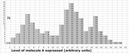
| 1D sample dataset . Here is a sample problem and KMM solution to introduce the idea more concretely.
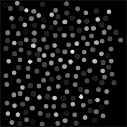
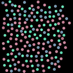
A fluorescence dataset reports the expression of a critical molecule A in a collection of cells. It is believed that three different cell classes are present in the sample. Does the fluorescence image of A visually report that segmentation? How many cell classes does it look like to you?
|
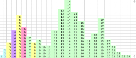
| 1D KMM. |
| 1D KMM Step 0. The KMM requires a single user input to begin: the number of expected classes K. The simplest implementation then picks K initial centers. Here we choose P(0) = 3, Q(0) = 5, and R(0) = 8 (yellow), but many implementations use automatic initiation. The initial task of the KMM is to assign the three classes based on Euclidian distance. Class P captures values ≤ 3 (blue) and shares half of the values between 3 and 5 (purple) with class Q. Class Q captures all values closer to 5 than 8 (red) and class R captures everything else (green).
|
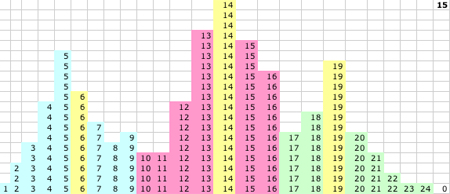
1D KMM Step 1. The KMM recalculates the K centers based on the new memberships in the classes and P(1)=3, Q(1)=5 and R(1)=15. R(1) is the only major revision at this step, but this radically changes the class memberships between R and Q.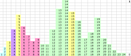 |
1D KMM Step 3. After a couple of cycles center Q starts to move.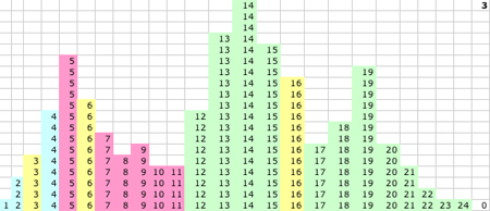 |
1D KMM Steps 0-15. The migrating means |
1D KMM Step 15. The KMM stops or converges on this solution:
|
| 1D KMM Theme Map. Using these values, we recode the original greyscale image according to class memberships P, Q, and R.
|
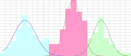
1D KMM & the Normal Distribution.
Separability is a more stringent measure than significance. If classes are truly separable with a small degree of error, they are explicitly significant. |