| Micromolecules: definitions & links | Cellular domains: Genome, preoteome & metabolome |
| Metabolic diversity: Scale, dynamics, & phyletics | Phenotyping strategies: proteomics vs metabolomics |
| CMP Platforms: Platforms and workflow overview | CMP Probes: The probe library |
| CMP Substrates: Molecular trapping & detection | CMP Datasets: Data arrays for multichannel imaging |
| CMP Analysis: pattern recognition theory and tools | CMP Exploration: N-space visualization tools |
| CMP Annotation: browsing & annotating data |
| IMAGE REGISTRATION TEST SETS |
| Raw, unregistered 8-bit tiff series |
| Details: Serial 250 nm resin tissue sections. Image capture resolution = 476 nm/pixel. Post-cap operations: INVERT Images with B, TT and E signals are easiest to align. G is the most difficult in this setCapture Series (Win: right-click > save as; Mac: Ctrl-click, save as) |
| Registered 8-bit tiff series |
| IMAGE CLASSIFICATION JEWEL SETS |
| IMAGE CLASSIFICATION WITH PCI |
| Files: full sized files 1350 x 964, 8-bits grey, background-masked, contrast-stretched 60-220 |
| Classification parameters PCI: Isodata, Clus(max 20, est 16, min 12), convergence 0.01, sample 20%, seed diagonal Morphias: Kmeans, 12 clus, sample 10%, seed random Theme Maps harmonized in GraphicConverter 5.6.2X for Mac OS 10.4 www.lemkesoft.com |
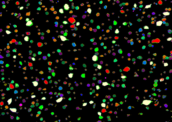 ↑ PCI = 11 classes Full size indexed tiff: Marc_2366_original_PCI_map.tif 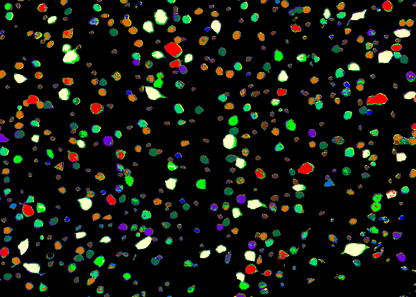 ↑ Morphias = 9 classes Full size indexed tiff: Marc_2366_morphias_map.tif 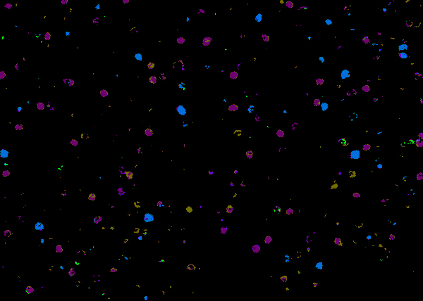 ↑ Morphias-PCI: The class match is excellent overall and argues that Morphias is already a good substitute for PCI. This is a difference map between Morphias and PCI (after median filtering to correct for some kerf errors). The purple class is a separate PCI class contained mostly within the orange class in Morphias. The blue class is a separate PCI class is contained mostly within the lite green class in Morphias. We compared some (not all) signals in CellKit as 2D histograms for these classes with the conclusion that PCI pushed the envelope a bit, while Morphias was conservative. Of course we restricted clusters to 12 and haven’t given Morphias a fair test yet. We also haven’t used mindis to assess separations. Maybe by the end of next week. Full size indexed tiff: Marc_2366_morphias-PCI_map.tif |
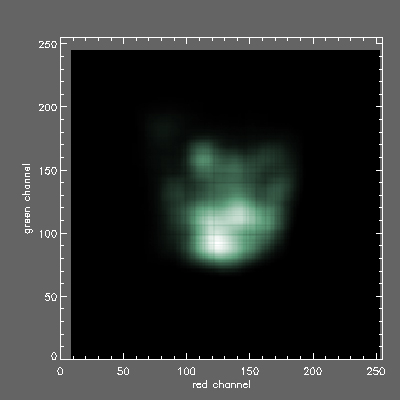
2D histogram of AGB (x axis red channel) vs GABA (y axis green channel) signals for the Morphias lite green class
2D histogram of AGB (x axis red channel) vs GABA (y axis green channel) signals for the PCI lite greenand blue classes with Morphias envelope. It seems that PCI was able to pick up the trough in signals between the modesDL TIFF file
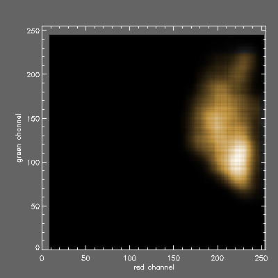
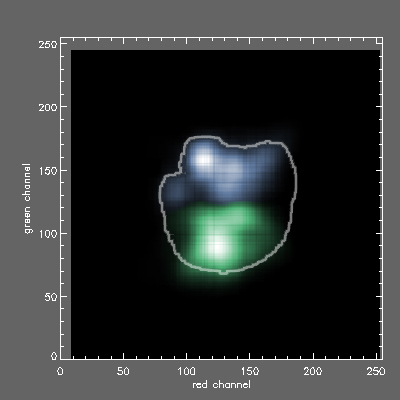
2D histogram of AGB (x axis red channel) vs GABA (y axis green channel) signals for the Morphias orange class

2D histogram of AGB (x axis red channel) vs GABA (y axis green channel) signals for the Morphias orange and purple classes with Morphias envelope. It seems that the Morphias outcome lumping all together is more defensible, although multiple modes are evident in the cluster.
Registered 8-bit tiff series
Reg
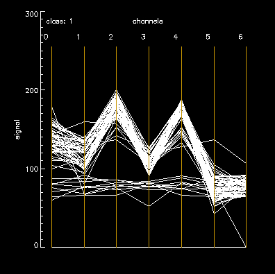
Classification “Noise” viewed in parallel plots with CellKit
| Registered 8-bit tiff series |
| Registered 8-bit tiff binary (0-255) cell object mask |
| 2546_small_masked_lo7_idl_thememask.tif |
| Registered 8-bit indexed Isodata classification result |
| 2546_small_masked_lo7_idl_themeindexed.tif |
Classification “Noise” viewed in parallel plots with CellKit
| Classification “Noise” viewed in parallel plots with CellKit
A parallel-plot algorithm reveals two “variance” sources our “refined” map for cell classes: intrinsic biological variance and outliers likely due to map misalignment. The plot is a polyline for each 7D point, connecting its partners on 7 parallel axes, for each class. Class 01 – noise = a sparse band of horizontal lines outside the main “M” shaped plot. SD=15 for class 01, channel 0 (chan_b).
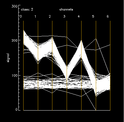
Class 2 – noise =a heavy band of horizontal lines ( a lot of bad pixels included under the mask) outside the main tilted “M” shaped plot. But SD is still only 8 for channel 0 (chan_b) because the density of “good” pixels is really high.
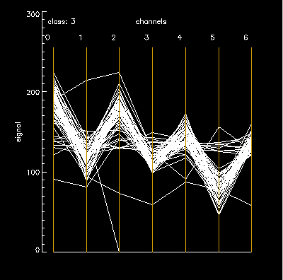
Class 3 – very few bad pixels, but the intrinsic dispersion is a little higher. (channel 0 SD =13) Obviously, the next thing to do is write an explore tool to highlight coordinates of the “bad” pixels in the polyline on the original image. |