| CellKit Downloads & Links |
| Cell Kit v2.2 for Win2K/XP IDL *.sav file for IDL 6.0 or greater VM (right-click: save-as) |
| Cell Kit v2.3 for OS X (X11) IDL *.sav file for IDL 6.1 or greater VM (right-click: save-as) |
| IDL 6.0 VM from RSI |
| CellKit Description and Full Help Files |
| CellKit (CK) is an application suite to explore classified or segmented images and visualize multivariate signatures of pre-aligned images such as multichannel datasets. CK was planned as a light-weight laboratory tool for our own biological research but is based on capabilities found in more powerful (and expensive) remote sensing application suites. The basic goals are to provide quick histogramming and classification tools for multichannel datasets. CK is early in its development (the interface and functions will undoubtedly change), but may be useful to those beginning their explorations of multichannel worlds. |
| CK was developed under IDL Versions 6.0 Win32 (x86) and 6.1, Mac OS X (X11 darwin ppc m32). This version is pre-compiled ‘ *.sav ‘ form that runs in the IDL Virtual Machine™ environment (© 2003 Research Systems, Inc). The IDL VM is a free application/environment for Windows, Unix and Mac OS X (X11) platforms. Link: IDL VM from RSI. |
| Overview
|
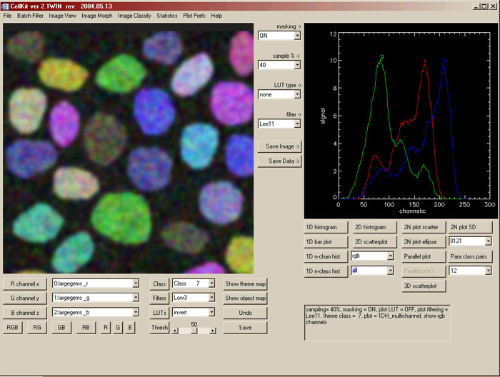
| CellKit displays, filters, histograms, scatterplots, N-plots and classifies data arrays from registered tiff files.
CellKit has five major fields (view the 1024 pixel interface): 1. The image view window (IW, left) where scaled images are displayed 2. The image view controls (lower left and center): 3. The data view window (DW, right) where multivariate data are visualized. 4. The data view controls (lower right): 5. The menu |
| Basic Functions | |
| Menu / Button / Droplist | Function |
| File > Preview Image | loads an image preview into the IW |
| File > Load Images | loads tiffs into the red, green and blue channel droplists |
| File > Load Theme Map | loads indexed tiff image into the class droplist |
| File > Load Object Mask | loads binary object mask tiff |
| File > Record Data Links | records all loaded image sets |
| File > Load Data Links | loads all recorded image sets |
| File > Exit | exits CK |
| Batch Filter > Filter Sequence | sets a sequence of up to 8 filters to apply to a file batch |
| Batch Filter > FilterSeq>Red | applies the filter sequence to the selected red [x] channel |
| Batch Filter > FilterSeq>All and Save | applies the filter to all loaded images and saves with new filenames |
| Batch Filter > FilterSeq>All, Save, Load | applies the filter to all loaded images, saves and reloads |
| Image Classify > Cluster | object-based quick classifier |
| Image Classify > Set Cluster Parameters | sets initial cluster and iteration numbers |
| Image Classify > Save Cluster Data | saves ASCII cluster data |
| Image Classify > Save Theme Map | saves classification theme map |
| Image Classify > Explore Theme Map | explore classification theme map |
| Plot Prefs> 1DH background | sets plot background to black or white |
| Plot Prefs> 1DH background | sets plot background to black or white |
| Plot Prefs> 2DS background | sets plot background to black or white |
| Plot Prefs> 3DS background | sets plot background to black or white |
| Plot Prefs> 2N background | sets plot background to black or white |
| Help > Help | help |
| Plot Prefs> Help > About CellKit | About CellKit |
| function & selection radio buttons | Function |
| show + R,G,B radio | loads grey images from the red, green or blue droplist |
| show + RGB radio | loads rgb image from all three droplists |
| show + Theme Map radio | loads an indexed image of the theme map |
| show + Theme Class radio | loads an indexed image of the theme class |
| show + Object Mask radio | loads an binary image of the object mask |
| filter + type & size radios | hi, lo, median or edge filters (3×3, 5×5, 7×7) of the displayed grey image |
| lut + type radios | stretch, equalization, inversion or slicer indexing of displayed grey image |
| save image | saves greyscale IW image at true size |
| show last | recovers last image (toggle) |
| percent radios | percent of the image to sample |
| mask checkbox | turn on class masking for all plots except 2N |
| equal checkbox | turn on histogram equalization for 2d and 3d hist |
| slicer checkbox | turn on slicer lut for 2d hist |
| filter radios | select ‘no’, ‘box’car or ‘lee’ (gaussian) filterting for 1d, 2d, 3d hist |
| run plot | runs data visualization with selected options |
| save plot | save ascii data |
| save image | save plot image as true color tiffy |
| plot type radios | Function |
| 1d hist | 1d hist of the red channel +/- theme class mask |
| 1d chan | 1d hist from ‘multichannel list’ channels +/- theme class mask |
| 1d class | 1d hist from ‘multiclass list’ & red channel droplist |
| 2d hist | 2d hist from x & y channels +/- theme class mask |
| 2d scatter | 2d scatterplot from x & y channels +/- theme class mask |
| 3d hist | 3dh of x, y, z channels +/- theme class mask (not implemented) |
| 3d scatter | 3d scatterplot from x, y & z channels +/- theme class mask |
| 2N plot | multi 2d scatterplots from ‘channel pairs’ +/- theme class mask |
| 2N op1 | multi 2d means + orthog 2sd channel pair ellipses +/-theme class mask |
| 2N op2 | multi 2d means + orthog 2sd channel pair ellipses +/-theme class mask |
| parallel | parallel plots from ‘multichannel’ and ‘multiclass’ list (not implemented) |
| droplists | Function |
| red channel [x] droplist | the image used for the x dimension in 1d, 2d and 3d plots |
| green channel [y] droplist | the image used for the y dimension in 2d and 3d plots |
| blue channel [z] droplist | the image used for the z dimension in 3d plots |
| theme class droplist | the class bitmask from the theme map |
| multichannel droplist | the list of channels for 1d chan plots |
| channel pairs droplist | the list of classes for 1d class plots |
| class pairs droplist | a list of pairwise classes (not implemented) |
| Basic Operations | |
| CK initial assumptions | |
| all data tiffs are are monochrome (1 channel) | |
| all tiffs are the same size | |
| all tiffs are registered | |
| theme map tiffs are properly indexed: 1 pixel value/class, starting at pixel value 0 | |
| Loading and Display | |
| 1. Only monochrome, single channel tiffs are accepted as input | |
| 2. Up to 96 tiffs may be selected, but only the first 16 are currently used | |
| 3. The display is rescaled but true image sizes are used in all operations | |
| Shortcuts to loading batches of files: using DataLinks | |
| To record a batch of files for future use… | |
| 1. Load any combination of images, theme maps and object masks | |
| 2. Select File > Record DataLinks and save as a *.dlk file | |
| To load a batch of recorded files … | |
| 1. Select File > Load DataLinks and select the desired *.dlk file | |
| As long as you do not move the files or rename directories, the DataLink will load them – even if you move the *.dlk. | |
| If some of the files have been moved, deleted, etc., DataLink will try to load the remainders | |
| Showing loaded images | |
| 1. Select the desired file in the red [x], green [y], blue [z] or theme class droplists | |
| 2. Select the desired radio (R,G,B, RGB, Theme Map, Theme Class or Object Mask) | |
| 3. Select ‘show’ | |
| NOTE: R,G,B are displayed as monochrome, RGB as rgb, all others as indexed | |
| Filtering displayed images | |
| 1. Select & show the desired monochrome (R,G,B) images | |
| 2. Select the desired filter and size radios | |
| 3. Select ‘filter’ | |
| 4. Select save image to save the displayed image as a new file at the original resolution | |
| NOTE: ‘filter’ operates on the displayed true-size image in memory, not disk files shown in the channel droplists | |
| NOTE: Filtering an image and re-selecting ‘show’ for that channel will undo all filters | |
| NOTE: Selecting ‘show last’ will undo the last filter. | |
| Filtering batches of images: will perform up to 8 serial filters on up to 16 files | |
| …set up the filter sequence | |
| 1. Select Batch Filter > Filter Sequence: select a string of 1-8 sequential filters to apply | |
| 2. Select ‘done’ | |
| …to test the filter sequence on an image | |
| 1. Select the desired file in the red channel [x] droplist | |
| 2. Select Batch Filter > Filter Seq>Red: filters and displays the result; save with ‘save image’ if desired | |
| …to filter all loaded images | |
| 1. Select Batch Filter > Filter Seq>All & Save: filters, appends ‘_batch.tif’ to the image name and saves | |
| WARNING: overwrites files already named ‘ *_batch.tif’. Use Filter Seq>All,Save,Load to avoid this. | |
| …to filter all loaded images and reload them for analysis | |
| 1. Select Batch Filter > Filter Seq>All, Save, Load: filters, appends ‘_batch.tif’, saves and reloads into droplists | |
| WARNING: click away willy-nilly and fill up a drive with ‘ *_batch_batch_batch.tif ‘ files! | |
| Viewing the display lut | |
| 1. Select & show the desired monochrome (R,G,B) images | |
| 2. Select the desired lut | |
| 3. Select ‘lut’ | |
| 4. Select save image to save the displayed image as a new file at the original resolution | |
| NOTE: ‘lut’ operates on the displayed true-size image in memory, not disk files shown in the channel droplists | |
| NOTE: Remapping an image and re-selecting ‘show’ for that channel will undo all filters | |
| NOTE: Selecting ‘show last’ will undo the last lut. | |
| GENERAL process to visualize signatures | |
| 1. Select plot type radio | |
| 2. Select the required droplist channels (red, green, blue) or multichannel etc | |
| 3. Select the class droplist (optional) | |
| 4. Select percent to sample the image (most operations require little data for accuracy, default =10%) | |
| 5. Select mask invoke the class droplist (optional, default=OFF) | |
| 6. Select equal and/or slicer to enhance 2d or 3d hist displays (optional, default=OFF) | |
| 7. Select filtering radios to operate on 1d, 2d, or 3d hist displays (default=no) | |
| 8. Select plot | |
| 9. Select save image to save the displayed plot as an rgb tiff | |
| 10. Select save plot to save plot data as an ascii file (not imlemented for all plot types) | |
| SPECIFIC processes to visualize signatures |
| 1d histogram signatures |
| 1. Select the ‘1d hist’ radio |
| 2. Select a file from the red channel [x] droplist |
| 3. Select a class from the theme class droplist (optional) |
| 4. Select percent to sample the image |
| 5. Select mask invoke the class droplist (optional) |
| 6. Select filtering radios |
| 7. Select plot |
| 8. Select ‘save image’ to save the displayed plot as an rgb tiff |
| 9. Select ‘save plot’ to save plot data as an ascii file |
| multichannel 1d histogram signatures |
| 1. Select the ‘1d chan’ radio |
| 2. Select a channel list from (or enter one into) the multichannel list |
| 3. Select a class from the theme class droplist (optional) |
| 4. Select percent to sample the image |
| 5. Select ‘mask’ invoke the class droplist (optional) |
| 6. Select filtering radios |
| 7. Select plot |
| 8. Select ‘save image’ to save the displayed plot as an rgb tiff |
| 9. Select ‘save plot’ to save plot data as an ascii file |
| 1d chan notes: select from existing options or enter your own values: 0-9, 10=a 11=b 12=c 13=d 14=e 15=f. Acceptable channel numbers are shown next to each file name in any channel droplist. Enter values as a list without spaces, commas, etc.: e.g. ‘123b5c’. If plot does not run, check the status line for an “illegal entry” error message. This suggests a text error in entering your list. |
| multiclass 1d histogram signatures |
| 1. Select the ‘1d class’ radio |
| 2. Select a class list from (or enter one into) the multiclass list |
| 3. Select a file from the red channel [x] droplist |
| 4. Select percent to sample the image |
| 5. Select filtering radios |
| 6. Select plot |
| 7. Select ‘save image’ to save the displayed plot as an rgb tiff |
| 8. Select ‘save plot’ to save plot data as an ascii file |
| 1d class list notes: select from existing options or enter your own values: 1-9, 10=a 11=b 12=c 13=d 14=e 15=f 16=g. Enter values as a list without spaces, commas, etc.: e.g. ‘123b5c’. If plot does not run, check the status line for an “illegal entry” error message. This suggests a text error in entering your list. |
| 2d histogram signatures |
| 1. Select the ‘2d hist’ radio |
| 2. Select files from the red channel [x] and green channel [y] droplists |
| 3. Select a class from the theme class droplist (optional) |
| 4. Select percent to sample the image |
| 5. Select ‘mask’ invoke the class droplist (optional) |
| 6. Select ‘equal’ to equalize the histogram (optional) |
| 7. Select ‘slicer’ to lut the histogram (optional) |
| 8. Select filtering radios |
| 9. Select plot |
| 10. Select ‘save image’ to save the displayed plot as an rgb tiff |
| 11. Select ‘save plot’ to save plot data as an ascii file |
| 2d hist notes: At low sampling percents, histograms visualized without equal or slicer may yield small noisy spots. |
| 2d scatterplot signatures |
| 1. Select the ‘2d scatter’ radio |
| 2. Select files from the red channel [x] and green channel [y] droplists |
| 3. Select a class from the theme class droplist (optional) |
| 4. Select percent to sample the image |
| 5. Select ‘mask’ invoke the class droplist (optional) |
| 6. Select plot |
| 7. Select ‘save image’ to save the displayed plot as an rgb tiff |
| 8. Select ‘save plot’ to save plot data as an ascii file |
| 2d scatter notes: At high sampling % on large images, time to plot may be long. |
| 3d histogram signatures not implemented |
| 3d scatterplot signatures |
| 1. Select the ‘3d scatter’ radio |
| 2. Select files from the red channel [x], green channel [y] and blue channel [z] droplists |
| 3. Select a class from the theme class droplist (optional) |
| 4. Select percent to sample the image |
| 5. Select ‘mask’ invoke the class droplist (optional) |
| 6. Select plot |
| 7. Select ‘save image’ to save the displayed plot as an rgb tiff |
| 8. Select ‘save plot’ to save plot data as an ascii file |
| 3d scatter notes: At high sampling % on large images, time to plot may be long. The dataset may be truncated and, if so, will be indicated on the status line |
| 2N plot signatures as scatterplots |
| 1. Select the ‘2N plot’ radio |
| 2. Select a list of channel pairs from (or enter one into) the channel pairs droplist |
| 3. Select a class from the theme class droplist (REQUIRED) |
| 4. Select percent to sample the image |
| 5. Select plot |
| 6. Select ‘save image’ to save the displayed plot as an rgb tiff |
| 9. Select ‘save plot’ to save plot data as an ascii file |
| 2N plot notes: select from existing options or enter your own values: 1-9, 10=a 11=b 12=c 13=d 14=e 15=f 16=g. Enter values as a list without spaces, commas, etc.: e.g. ‘123b5c’. The list is interpreted as a sequence of ‘x vs y’ pairs. Channel numbers may be replicated as desired. If plot does not run, check the status line for an “illegal entry” error message. This suggests a text error in entering your list. |
| 2N plot signatures as means with 2sd ellipses – plotted as orthogonal sds |
| 1. Select the ‘2N op1’ radio |
| 2. Select a list of channel pairs from (or enter one into) the channel pairs droplist |
| 3. Select a class from the theme class droplist (REQUIRED) |
| 4. Select percent to sample the image |
| 5. Select plot |
| 6. Select ‘save image’ to save the displayed plot as an rgb tiff |
| 9. Select ‘save plot’ to save plot data as an ascii file |
| 2N op1 plot notes: select from existing options or enter your own values: 1-9, 10=a 11=b 12=c 13=d 14=e 15=f 16=g. Enter values as a list without spaces, commas, etc.: e.g. ‘123b5c’. The list is interpreted as a sequence of ‘x vs y’ pairs. Channel numbers may be replicated as desired. If plot does not run, check the status line for an “illegal entry” error message. This suggests a text error in entering your list. |
| 2N plot signatures as means with 2sd ellipses – plotted as tilted sds calculated from gaussian fits |
| 1. Select the ‘2N op2’ radio |
| 2. Select a list of channel pairs from (or enter one into) the channel pairs droplist |
| 3. Select a class from the theme class droplist (REQUIRED) |
| 4. Select percent to sample the image |
| 5. Select plot |
| 6. Select ‘save image’ to save the displayed plot as an rgb tiff |
| 9. Select ‘save plot’ to save plot data as an ascii file |
| 2N op1 plot notes: select from existing options or enter your own values: 1-9, 10=a 11=b 12=c 13=d 14=e 15=f 16=g. Enter values as a list without spaces, commas, etc.: e.g. ‘123b5c’. The list is interpreted as a sequence of ‘x vs y’ pairs. Channel numbers may be replicated as desired. If plot does not run, check the status line for an “illegal entry” error message. This suggests a text error in entering your list. |
| Parallel plot signatures not implemented |
| Classifying Images |
| 1. Load images |
| 2. Load an object mask |
| 3. Select File > Image Classify > Set Cluster Parameters to change if desired |
| 4. Select File > Image Classify > Cluster Image |
| 5. Select File > Image Classify > Save Cluster Data if desired |
| 6. Select File > Image Classify > Save Theme Map to save the displayed plot as an indexed tiff |
| 9. Select File > Image Classify > Explore Theme Map to browse the data |
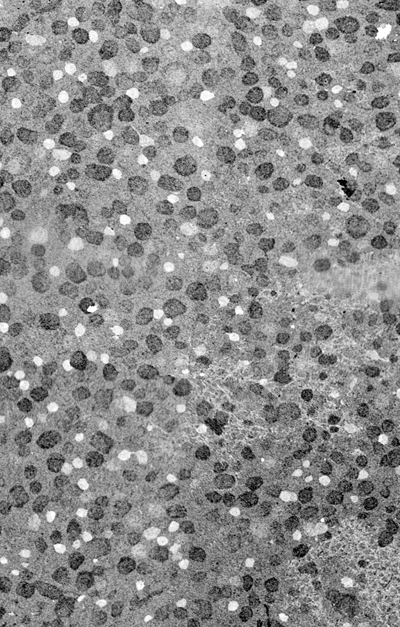
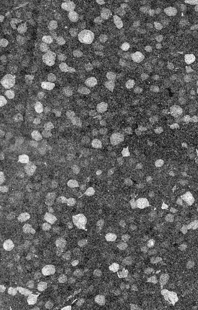
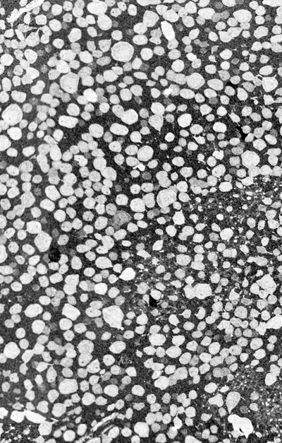
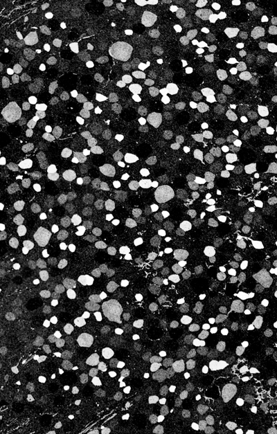
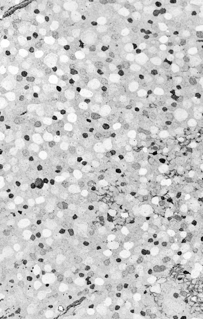
Example Images
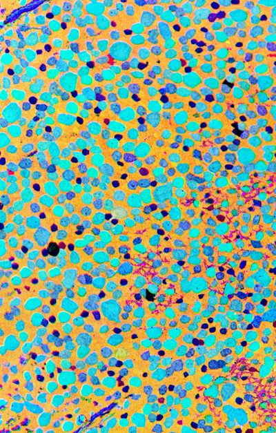
RGB = tt.q.e
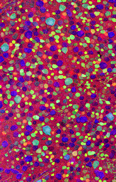
RGB = g.yy.tt
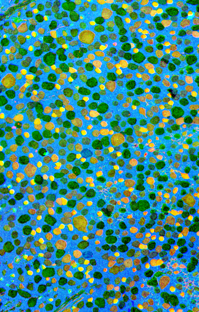
RGB = yy.a.d
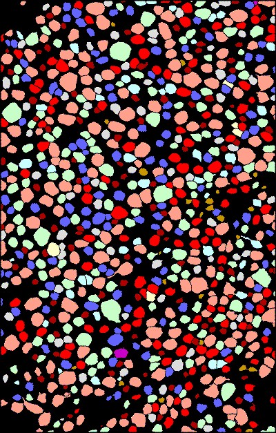
CELLKIT OBJECT THEME MAP
Alanine
Aspartate
Glutamate

Glycine
GABA
Glutamine

Taurine
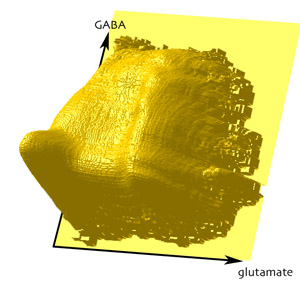
EY Surface
Legal
| This is a pre-release version for laboratory investigation only. It is not certified as a clinical, forensic, or policy tool. The code is not optimized for system performance. We aren’t responsible for what you do with it or what happens when you use it. That may be obvious, but we have to say it these days. CK may be freely distributed as long as the original copyright is included. Bugs, requests for features, etc may be reported to bryan.jones@m.cc.utah.edu. |